Full guide to Linear Regression (Part 2)

Linear Regression in 2 dimensions

So far, we have covered the unidimensional linear regression framework. But as you might expect, this is only a simple version of the linear regression model. Back to our housing price problem. So far, we only included the GPD variable. But as you may know, interest rates are also major leverage on the housing market.

Framework

The more general framework can be described as : \(Y = X {\beta}+ {\epsilon}\) . Notice that we are now in matrix form. Indeed :

• we suppose we have n observations of a dataset and p features per observation
• \(Y\) is the output of this observation
• \({\beta}\) is the column vector that contains the true parameters
• \(X\) is now a matrix of dimension (nxp)

Otherwise, the conditions on \({\epsilon}\) remain the same.

• \(E({\epsilon}) = 0\) , i.e a white noise condition
• \({\epsilon}_i ∼ iid {\epsilon}\) for all i = 1,…,n, i.e a homoskedasticity condition

In the 2 dimension problem introduced above to predict the housing prices, our task is now to estimate the following model : \(\hat{Y}_i = \hat{\beta}_0 + \hat{\beta}_1{X}_{1i} + \hat{\beta}_2{X}_{2i}\)

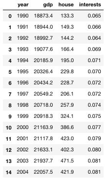
The dataset I’m using can be found here.

import pandas as pd
import numpy as np
import math

df = pd.read_csv('https://maelfabien.github.io/myblog/files/housing.txt', sep=" ")
df

fig, axs = plt.subplots(2, figsize=(8,8))

axs[0].scatter(df['gdp'], df['house'])
axs[1].scatter(df['interests'], df['house'], c='r')

axs[0].set_xlabel("Gross Domestic Product", fontsize = 12)
axs[0].set_ylabel("Housing Price", fontsize = 12)
axs[0].set_title("Relation between GDP and Average Housing Prices")

axs[1].set_xlabel("Interest rates", fontsize = 12)
axs[1].set_ylabel("Housing Price", fontsize = 12)
axs[1].set_title("Relation between interest rates and Average Housing Prices")

plt.tight_layout()

plt.show()

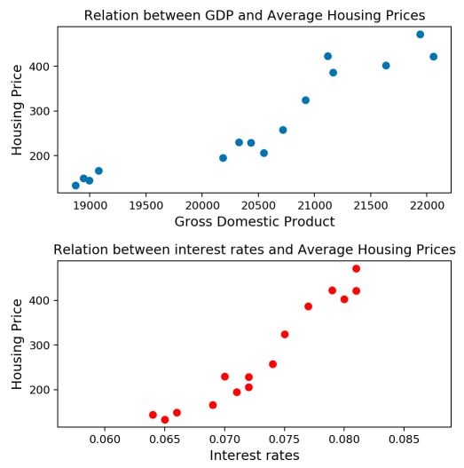
The linear relationship with the interest rate seems to hold again! Let’s dive into the model.

OLS estimate

Recall that to estimate the parameters, we want to minimize the sum of squared residuals. In the higher dimension, the minimization problem is :

\(argmin \sum(Y_i - X \hat{\beta})^2\) .

In our specific example, \(argmin \sum(Y_i - \hat{\beta}_0 - \hat{\beta}_1 {X}_{1i} - \hat{\beta}_2 {X}_{2i})^2\)

The general solution to OLS is : \(\hat{\beta} = {(X^TX)^{-1}X^TY}\) . Simply remember that this solution can only be derived if the Gram matrix defined by \(X^TX\) is invertible. Equivalently, \(Ker(X) = {0}\) . This condition guarantees the uniqueness of the OLS estimator.

x = np.hstack([np.ones(shape=(len(y), 1)), df[['gdp', 'interests']]]).astype(float)
xt = x.transpose()
X_gram = x
gram = np.matmul(xt, x)
i_gram = inv(gram)

We can use the Gram matrix to compute the estimator \(\hat{\beta}\) :

Beta = np.matmul(inv(gram), np.matmul(xt,y))

#Display coefficients Beta0, Beta1 and Beta2
print("Estimator of Beta0 : " + str(round(Beta[0],4)))
print("Estimator of Beta1 : " + str(round(Beta[1],4)))
print("Estimator of Beta2 : " + str(round(Beta[2],4)))

Estimator of Beta0 : -1114.2614 Estimator of Beta1 : -0.0079 Estimator of Beta2 : 21252.7946

We will discuss cases in which this condition is not met in the next article.

Orthogonal projection

Note that \(\hat{Y} = X \hat{\beta} = X(X^TX)^{-1}X^TY = H_XY\) where \(H_X = X(X^TX)^{-1}X^T\) . We say that \(H_X\) is an orthogonal projector since it meets two conditions :

• \(H_X\) is symmetrical : \({H_X}^T = H_X\)
• \(H_X\) is idempotent : \({H_X}^2 = H_X\)

Graphically, this projection states that we project \(\hat{Y}\) onto the hyperplane formed by the columns of X.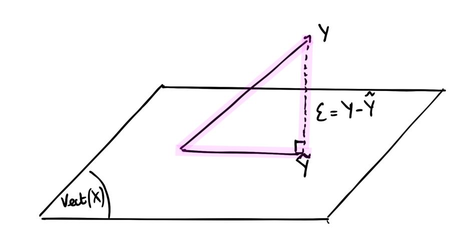

This allows us to redefine the vectors of residuals : \({\epsilon} = Y - \hat{Y} = (I - H_X)Y\) where \(I\) is the identity matrix.

\((I - H_X)\) is an orthogonal projector on the orthogonal of \(Vect(X)\) .

Bias and Variance of the parameters

Notice that \(\hat{\beta} - {\beta} = (X^TX)^{-1}X^TY - (X^TX)^{-1}X^TX{\beta} = (X^TX)^{-1}X^T{\epsilon}\)

The bias of the parameter is defined by : \(E(\hat{\beta}) - {\beta} = E(\hat{\beta} - {\beta}) = E((X^TX)^{-1}X^T{\epsilon}) = (X^TX)^{-1}X^TE({\epsilon}) = 0\) . The estimate \(\hat{\beta}\) of the parameter \({\beta}\) is unbiaised.

The variance of the parameter is given by : \(Cov(\hat{\beta}) = (X^TX)^{-1}X^TCov({\epsilon})X(X^TX)^{-1} = (X^TX)^{-1}{\sigma}^2\) . Therefore, for each \({\beta}_j\) : \(\hat{\sigma}^2_j = \hat{\sigma}^2{(X^tX)^{-1}_{j,j}}\)

#Standard errors of the coefficients
sigma = math.sqrt(((y - Beta[0] - Beta[1] * xt[1] - Beta[2]*xt[2])**2).sum()/(len(y)-3))
sigma2 = sigma ** 2

se_beta0 = math.sqrt(sigma2 * inv(gram)[0,0])
se_beta1 = math.sqrt(sigma2 * inv(gram)[1,1])
se_beta2 = math.sqrt(sigma2 * inv(gram)[2,2])

print("Estimator of the standard error of Beta0 : " + str(round(se_beta0,3)))
print("Estimator of the standard error of Beta1 : " + str(round(se_beta1,3)))
print("Estimator of the standard error of Beta2 : " + str(round(se_beta2,3)))

Estimator of the standard error of Beta0 : 261.185 Estimator of the standard error of Beta1 : 0.033 Estimator of the standard error of Beta2 : 6192.519

The significance of each variable is assessed using an hypothesis test : \(\hat{T}_j = \frac{\hat{\beta}_j} {\hat{\sigma}_j}\)

#Student t-stats
t0 = Beta[0]/se_beta0
t1 = Beta[1]/se_beta1
t2 = Beta[2]/se_beta2
print("T-Stat Beta0 : " + str(round(t0,3)))
print("T-Stat Beta1 : " + str(round(t1,3)))
print("T-Stat Beta2 : " + str(round(t2,3)))

T-Stat Beta0 : -4.266 T-Stat Beta1 : -0.242 T-Stat Beta2 : 3.432

Something pretty interesting happens here: by adding a new variable to the model, the coefficient of \({\beta}_1\) quite logically changed but became non-significant. We do expect \({\beta}_2\) to explain the model way better now.

The Quadratic Risk is : \(E[(\hat{\beta} - {\beta})^2] = {\sigma}^2 \sum{\lambda}_k^{-1}\) where \({\lambda}_k\) are the eigenvalues of the Gram matrix.

The prediction risk is : \(E[(\hat{Y} - Y)^2] = {\sigma}^2 (p+1)\)

The Github repository of this article can be found here.